The second part of this analysis will include EDA, feature selection, and finally creating some subset data to push to Tableau for building a dashboard. This will show comparisons between overall and Quentin Tarantino. Simple EDA charts and feature selection with the use of machine learning to explore and extract key information from the data.

Load Libraries

from pyspark.sql import SparkSession
import pandas as pd
import yaml
import os
import matplotlib.pyplot as plt
import numpy as np
import seaborn as sns

Create Spark Session and Create SQL Table

from pyspark.sql import SparkSession
from pyspark.sql.utils import AnalysisException
import os

try:
    # Initialize Spark session
    print("Initializing Spark session...")
    spark = SparkSession.builder \
        .appName("movies_db") \
        .config("spark.jars", "/usr/local/spark/jars/postgresql-42.7.4.jar") \
        .config("spark.driver.extraClassPath", "/usr/local/spark/jars/postgresql-42.7.4.jar") \
        .getOrCreate()

    print("Spark session created successfully.")


    # Define the CSV file path
    csv_file = "./imbd_movies.csv"  # Update with the correct path

    # Check if the CSV file exists
    if not os.path.exists(csv_file):
        raise FileNotFoundError(f"CSV file not found at path: {csv_file}")

    # Read CSV file into DataFrame
    print(f"Attempting to read CSV file from path: {csv_file}")
    df = spark.read.csv(csv_file, header=True, inferSchema=True)
    print("CSV file read successfully.")

    # Create a temporary view for SQL queries
    df.createOrReplaceTempView("movies")
    print("Temporary view 'movies' created successfully.")

except AnalysisException as e:
    print(f"AnalysisException: {e}")
except FileNotFoundError as e:
    print(f"FileNotFoundError: {e}")
except Exception as e:
    print(f"An error occurred: {e}")

Initializing Spark session...
Spark session created successfully.
Attempting to read CSV file from path: ./imbd_movies.csv
CSV file read successfully.
Temporary view 'movies' created successfully.

Here shows the connection to the spark container. The IMBD Movies dataset is inside the container. This was mounted by the inital docker run commmand to use my local directory inside the container. Doing it this way, makes the process easier than moving the dataset inside.

TOP 10 Rows

movies = spark.sql("""
    SELECT *
    FROM movies
    LIMIT 10
""")

movies.toPandas()

	Best Picture	Certificate (GB)	Certificate (US)	Color	Contains Genre?	Contains Production Company?	Continent	Country	Genres (1st)	Genres (2nd)	...	Title Id	What did they do ?	Who did they play ?	Year of Release	Billing (position in cast list)	IMDB Rating	Number of people	Number of titles	Number Of Votes	Runtime (Minutes)
0	None	None	None	None	None	None	None	None	None	None	...	tt0193499	actor	None	1952	1	None	1	1	None	None
1	None	None	None	None	None	False	None	None	None	None	...	tt0193293	actor	Lam Tsi-King	1954	1	None	1	1	None	None
2	None	None	None	None	None	False	None	None	None	None	...	tt0245957	actor	None	1961	1	None	1	1	None	None
3	None	None	None	None	None	None	None	None	None	None	...	tt0247371	actor	Sculptor Martin	1965	1	None	1	1	None	None
4	None	None	None	None	None	None	None	None	None	None	...	tt0498914	actor	Jagga	1992	1	None	1	1	None	132
5	None	None	None	None	None	None	None	None	None	None	...	tt6448596	actor	Sakir	2007	1	1.8	1	1	61	95
6	None	None	None	None	None	None	None	None	None	None	...	tt0205040	actor	Ng Chi Keung	1952	2	None	1	1	None	None
7	None	None	None	None	None	None	None	None	None	None	...	tt0192202	actor	None	1953	2	None	1	1	None	None
8	None	None	None	None	None	False	None	None	None	None	...	tt0192049	actor	None	1953	2	None	1	1	None	None
9	None	None	None	None	None	False	None	None	None	None	...	tt0193153	actor	None	1958	2	None	1	1	None	None

10 rows × 37 columns

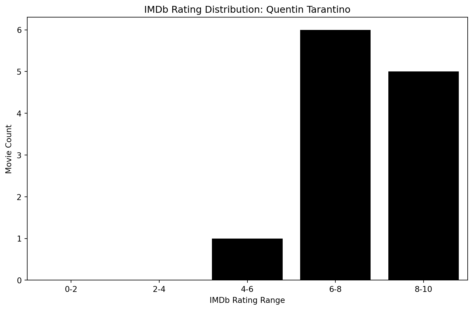
Distribution Comparison: Overall vs Quentin Tarintino

# Rating distribution for all directors
all_directors_ratings = spark.sql("""
    SELECT 
        CASE 
            WHEN CAST(`IMDB Rating` AS FLOAT) BETWEEN 0 AND 2 THEN '0-2'
            WHEN CAST(`IMDB Rating` AS FLOAT) BETWEEN 2 AND 4 THEN '2-4'
            WHEN CAST(`IMDB Rating` AS FLOAT) BETWEEN 4 AND 6 THEN '4-6'
            WHEN CAST(`IMDB Rating` AS FLOAT) BETWEEN 6 AND 8 THEN '6-8'
            WHEN CAST(`IMDB Rating` AS FLOAT) BETWEEN 8 AND 10 THEN '8-10'
        END AS rating_range, 
        COUNT(*) AS movie_count
    FROM movies
    WHERE `What did they do ?` = 'director'
    GROUP BY rating_range
    ORDER BY rating_range
""")

# Rating distribution for Quentin Tarantino's movies
tarantino_ratings = spark.sql("""
    SELECT 
        CASE 
            WHEN CAST(`IMDB Rating` AS FLOAT) BETWEEN 0 AND 2 THEN '0-2'
            WHEN CAST(`IMDB Rating` AS FLOAT) BETWEEN 2 AND 4 THEN '2-4'
            WHEN CAST(`IMDB Rating` AS FLOAT) BETWEEN 4 AND 6 THEN '4-6'
            WHEN CAST(`IMDB Rating` AS FLOAT) BETWEEN 6 AND 8 THEN '6-8'
            WHEN CAST(`IMDB Rating` AS FLOAT) BETWEEN 8 AND 10 THEN '8-10'
        END AS rating_range, 
        COUNT(*) AS movie_count
    FROM movies
    WHERE `Person Name` = 'Quentin Tarantino' AND `What did they do ?` = 'director'
    GROUP BY rating_range
    ORDER BY rating_range
""")

# Convert to pandas for plotting
all_directors_df = all_directors_ratings.toPandas()
tarantino_df = tarantino_ratings.toPandas()

The overall IMBD Rating has ratings starting from the 0-2 bin to the 8-10 bin. Compared to Tarantino, his lowest rating bin starts at the 4-6 bin. This is one film. However, he has six films in the 6-8 bin and 5 films in the 8-10 bin.

import matplotlib.pyplot as plt
import seaborn as sns

# Add a 'Director' column to distinguish between all directors and Quentin Tarantino
all_directors_df['Director'] = 'All Directors'
tarantino_df['Director'] = 'Quentin Tarantino'

# Reset index to avoid duplicate index issues when concatenating
all_directors_df = all_directors_df.reset_index(drop=True)
tarantino_df = tarantino_df.reset_index(drop=True)

# Sort the combined dataframe by 'rating_range' to ensure proper ordering in the plot
rating_order = ['0-2', '2-4', '4-6', '6-8', '8-10']
all_directors_df['rating_range'] = pd.Categorical(all_directors_df['rating_range'], categories=rating_order, ordered=True)
tarantino_df['rating_range'] = pd.Categorical(tarantino_df['rating_range'], categories=rating_order, ordered=True)

# Create separate figures for each plot

# Plot for All Directors
plt.figure(figsize=(10, 6))
sns.barplot(data=all_directors_df, x='rating_range', y='movie_count', color='darkgrey')
plt.xlabel('IMDb Rating Range')
plt.ylabel('Movie Count')
plt.title('IMDb Rating Distribution: All Directors')
plt.show()

# Plot for Quentin Tarantino
plt.figure(figsize=(10, 6))
sns.barplot(data=tarantino_df, x='rating_range', y='movie_count', color='k')
plt.xlabel('IMDb Rating Range')
plt.ylabel('Movie Count')
plt.title('IMDb Rating Distribution: Quentin Tarantino')
plt.show()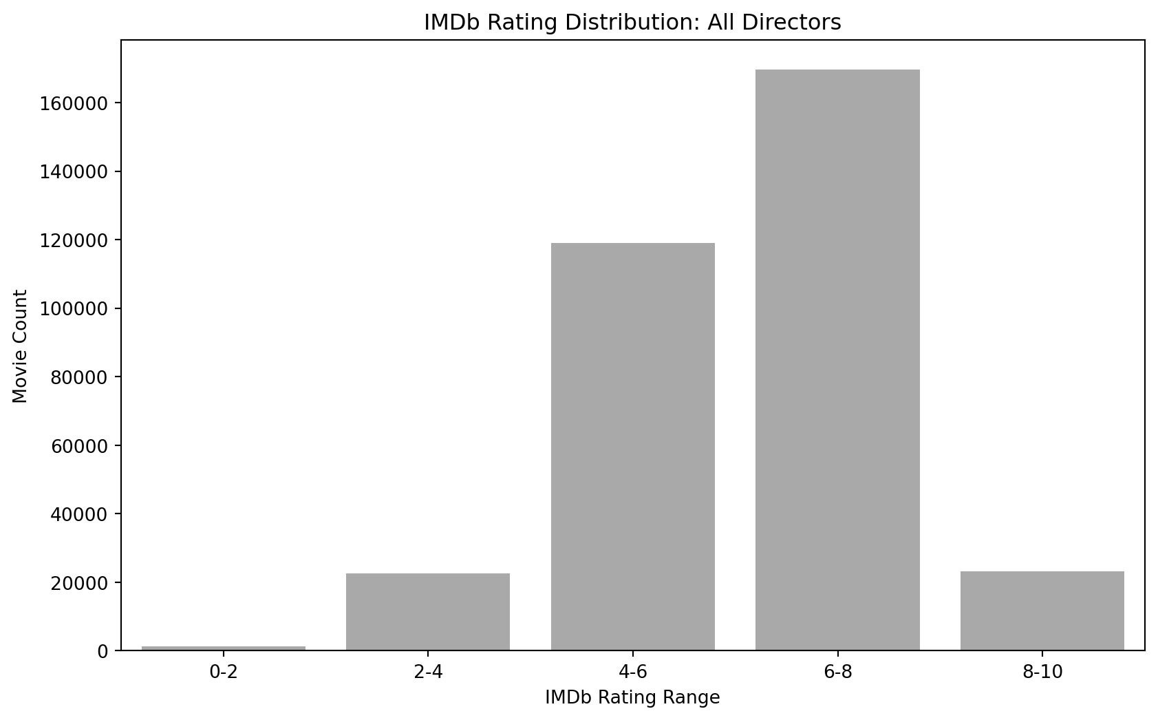

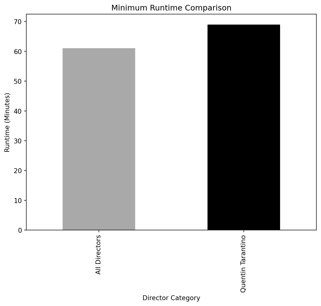
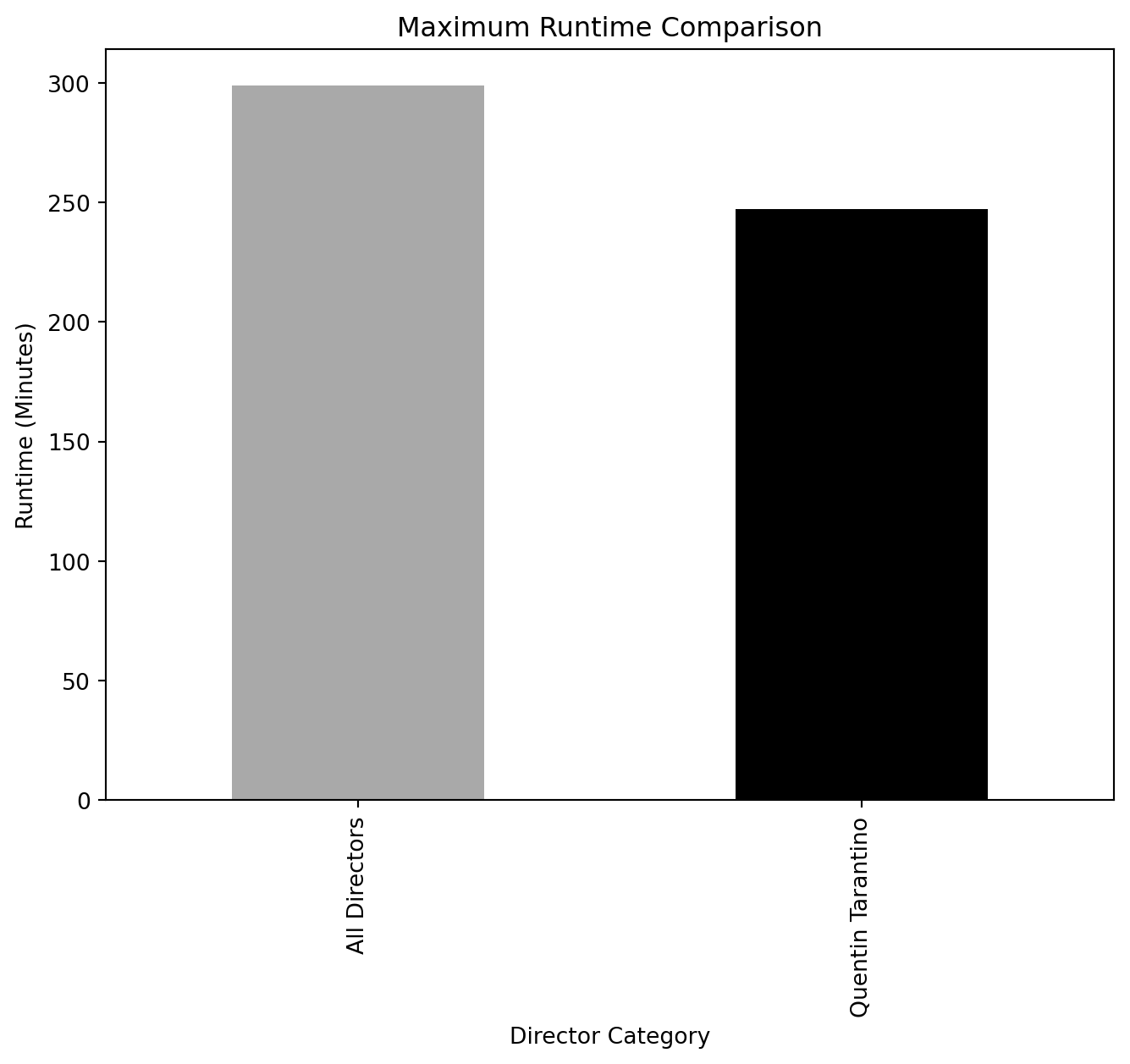
Runtime Comparison (Overall vs. Quentin Tarantino)

overall_runtime_stats = spark.sql("""
    SELECT 
        AVG(CAST(`Runtime (Minutes)` AS FLOAT)) AS avg_runtime,
        MIN(CAST(`Runtime (Minutes)` AS FLOAT)) AS min_runtime,
        MAX(CAST(`Runtime (Minutes)` AS FLOAT)) AS max_runtime
    FROM movies
    WHERE `What did they do ?` = 'director' AND `Runtime (Minutes)` < 300 AND `Runtime (Minutes)` > 60
""")


tarantino_runtime_stats = spark.sql("""
    SELECT 
        AVG(CAST(`Runtime (Minutes)` AS FLOAT)) AS avg_runtime,
        MIN(CAST(`Runtime (Minutes)` AS FLOAT)) AS min_runtime,
        MAX(CAST(`Runtime (Minutes)` AS FLOAT)) AS max_runtime
    FROM movies
    WHERE `Person Name` = 'Quentin Tarantino' AND `What did they do ?` = 'director' AND `Runtime (Minutes)` < 300 AND `Runtime (Minutes)` > 60
""")




overall_runtime_df = overall_runtime_stats.toPandas()
tarantino_runtime_df = tarantino_runtime_stats.toPandas()

import pandas as pd
import matplotlib.pyplot as plt

# Sample data assuming the data from `overall_runtime_df` and `tarantino_runtime_df` is available
runtime_data = {
    "Director": ["All Directors", "Quentin Tarantino"],
    "Avg Runtime": [overall_runtime_df['avg_runtime'][0], tarantino_runtime_df['avg_runtime'][0]],
    "Min Runtime": [overall_runtime_df['min_runtime'][0], tarantino_runtime_df['min_runtime'][0]],
    "Max Runtime": [overall_runtime_df['max_runtime'][0], tarantino_runtime_df['max_runtime'][0]]
}

runtime_df = pd.DataFrame(runtime_data)

# Separate plots for each metric
metrics = ["Avg Runtime", "Min Runtime", "Max Runtime"]
titles = ["Average Runtime Comparison", "Minimum Runtime Comparison", "Maximum Runtime Comparison"]

for metric, title in zip(metrics, titles):
    runtime_df.plot(x='Director', y=metric, kind="bar", legend=False, color=['darkgray', 'k'], figsize=(8, 6))
    plt.title(title)
    plt.ylabel("Runtime (Minutes)")
    plt.xlabel("Director Category")
    plt.show()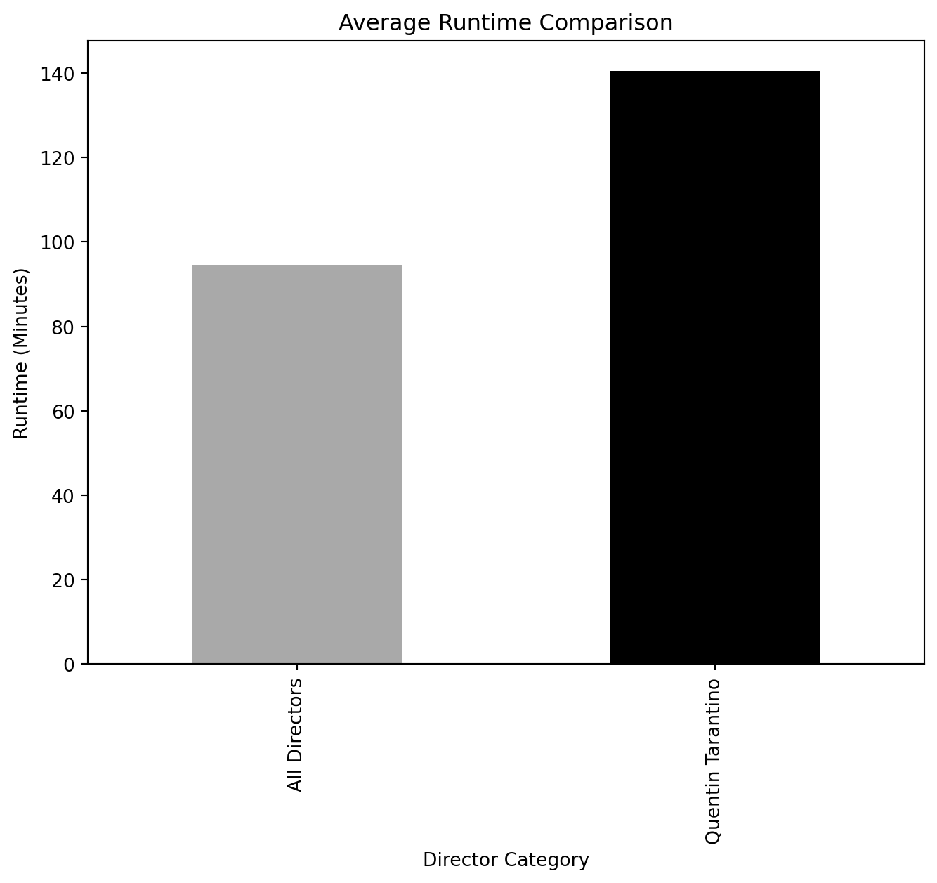

Genre Comparison: (Overall vs. Quentin Tarantino)

import matplotlib.pyplot as plt
import seaborn as sns
import numpy as np

# Retrieve genre distributions from Spark SQL
tarantino_genres = spark.sql("""
    SELECT genre, COUNT(*) AS genre_count
    FROM (
        SELECT EXPLODE(SPLIT(`Genres (full list)`, ',')) AS genre
        FROM movies
        WHERE `Person Name` = 'Quentin Tarantino'
    ) AS tarantino_genres
    GROUP BY genre
    ORDER BY genre_count DESC
""")

all_genres = spark.sql("""
    SELECT genre, COUNT(*) AS genre_count
    FROM (
        SELECT EXPLODE(SPLIT(`Genres (full list)`, ',')) AS genre
        FROM movies
    ) AS all_genres
    GROUP BY genre
    ORDER BY genre_count DESC
""")

# Convert the results to pandas DataFrames for plotting
tarantino_genres_df = tarantino_genres.toPandas()
all_genres_df = all_genres.toPandas()

# Add a 'Director' column to differentiate the datasets
tarantino_genres_df['Director'] = 'Quentin Tarantino'
all_genres_df['Director'] = 'All Directors'

# Combine both DataFrames into one for easier plotting
combined_df = pd.concat([tarantino_genres_df, all_genres_df])

# Sort the combined DataFrame by genre count in descending order
combined_df = combined_df.sort_values(by='genre_count', ascending=False)

# Set up the plot
plt.figure(figsize=(12, 8))

log_y = np.log(combined_df['genre_count'])
# Create the bar plot with proper dodge to prevent overlap
sns.barplot(data=combined_df, x='genre', y=log_y, hue='Director', palette=['k', 'darkgrey'])

# Rotate the x-axis labels for better readability
plt.xticks(rotation=90)

# Add labels and title
plt.xlabel('Genre')
plt.ylabel('Movie Count')
plt.title('Genre Distribution: Quentin Tarantino vs All Directors (Log Scale)')
plt.legend(title="Director Category")

# Show the plot
plt.tight_layout()
plt.show();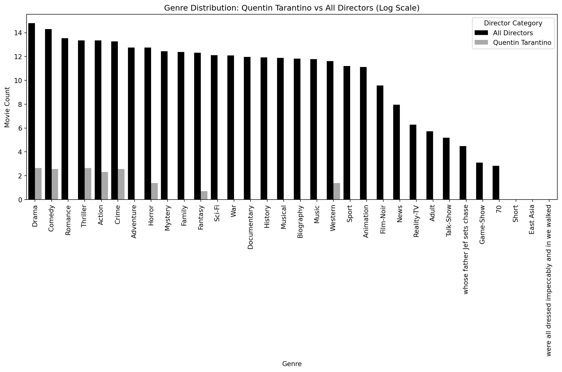

Production Company Comparison: (TOP 10 Overall vs. Quentin Tarantino)

# General production company distribution for all directors
production = spark.sql("""
    SELECT 
        `Production Companies (1st)` AS production_company, 
        COUNT(*) AS movie_count
    FROM movies
    WHERE `What did they do ?` = 'director' AND `Production Companies (List)` IS NOT NULL
    GROUP BY production_company
    ORDER BY movie_count DESC
    LIMIT 10
""")

# Production companies for Quentin Tarantino
production_qt = spark.sql("""
    SELECT 
        `Production Companies (1st)` AS production_company, 
        COUNT(*) AS movie_count
    FROM movies
    WHERE `Person Name` = 'Quentin Tarantino' AND `What did they do ?` = 'director' AND `Production Companies (List)` IS NOT NULL
    GROUP BY production_company
    ORDER BY movie_count DESC
""")

# Convert Spark DataFrames to Pandas DataFrames
tarantino_production_df = production_qt.toPandas()
all_production_df = production.toPandas()

# Create comparison plots
import matplotlib.pyplot as plt
import seaborn as sns

# Add a 'Director' column to each DataFrame to differentiate
tarantino_production_df['Director'] = 'Quentin Tarantino'
all_production_df['Director'] = 'All Directors'

# Combine both DataFrames into one for easier plotting
combined_production_df = pd.concat([tarantino_production_df, all_production_df])

# Set up the plot
plt.figure(figsize=(12, 8))

# Create a bar plot with production companies on the x-axis and movie count on the y-axis
sns.barplot(data=combined_production_df, x='production_company', y='movie_count', hue='Director', palette=['k', 'darkgrey'])

# Apply a logarithmic scale to the y-axis
plt.yscale('log')

# Rotate x-axis labels for readability
plt.xticks(rotation=45, ha='right')

# Add labels and title
plt.xlabel('Production Company')
plt.ylabel('Log of Movie Count')
plt.title('Top Production Companies: Quentin Tarantino vs All Directors')
plt.legend(title="Director Category")

# Show plot
plt.tight_layout()
plt.show()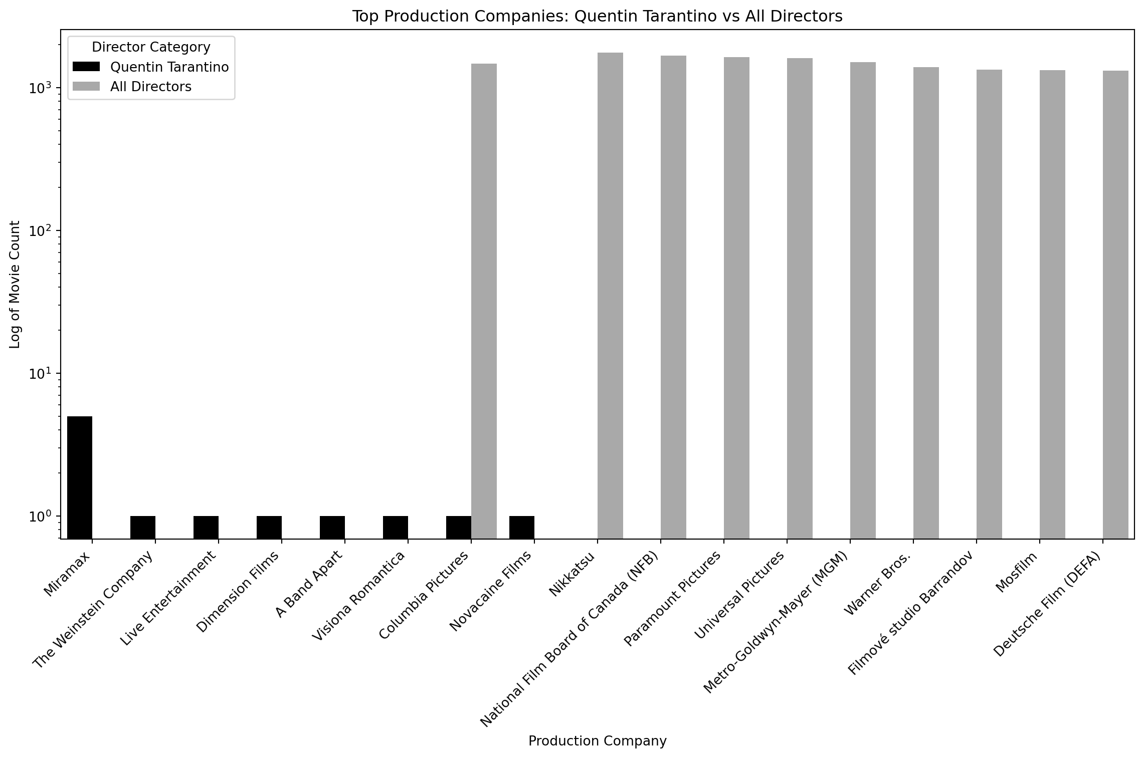

Time-Series: Average Imbd Rating (Overall vs. Quentin Tarantino)

tarantino_yearly = spark.sql("""
    SELECT 
        CAST(`Year of Release` AS INT) AS year,
        COUNT(*) AS movie_count,
        AVG(CAST(`IMDB Rating` AS FLOAT)) AS avg_rating
    FROM movies
    WHERE `Person Name` = 'Quentin Tarantino' AND `What did they do ?` = 'director'
    GROUP BY year
    ORDER BY year
""")

all_directors_yearly = spark.sql("""
    SELECT 
        CAST(`Year of Release` AS INT) AS year,
        COUNT(*) AS movie_count,
        AVG(CAST(`IMDB Rating` AS FLOAT)) AS avg_rating
    FROM movies
    WHERE `What did they do ?` = 'director'
    GROUP BY year
    ORDER BY year
""")

# Convert Spark DataFrames to pandas
tarantino_yearly_df = tarantino_yearly.toPandas()
all_directors_yearly_df = all_directors_yearly.toPandas()

# Add 'Director' column to distinguish in plotting
tarantino_yearly_df['Director'] = 'Quentin Tarantino'
all_directors_yearly_df['Director'] = 'All Directors'

# Combine DataFrames
combined_yearly_df = pd.concat([tarantino_yearly_df, all_directors_yearly_df])

# Check for any missing values in the DataFrame
#print(combined_yearly_df.isna().sum())

# Drop rows with missing values if any
combined_yearly_df.dropna(subset=['year', 'avg_rating'], inplace=True)

# Ensure 'year' is integer type and 'avg_rating' is numeric
combined_yearly_df['year'] = combined_yearly_df['year'].astype(int)
combined_yearly_df['avg_rating'] = pd.to_numeric(combined_yearly_df['avg_rating'], errors='coerce')

# Check if any non-numeric data slipped into 'avg_rating' and convert to numeric again if necessary
combined_yearly_df.dropna(subset=['avg_rating'], inplace=True)

# Try plotting again
import matplotlib.pyplot as plt
import seaborn as sns

plt.figure(figsize=(10, 6))

# Plot number of movies per year
plt.subplot(2, 1, 1)
sns.lineplot(data=combined_yearly_df, x='year', y='movie_count', hue='Director', marker='o',palette=['k', 'darkgrey'])
plt.xlabel('Year')
plt.ylabel('Number of Movies')
plt.title('Number of Movies Released Per Year: Quentin Tarantino vs All Directors')

# Plot average IMDb rating per year
plt.subplot(2, 1, 2)
sns.lineplot(data=combined_yearly_df, x='year', y='avg_rating', hue='Director', marker='o', palette=['k', 'darkgrey'])
plt.xlabel('Year')
plt.ylabel('Average IMDb Rating')
plt.title('Average IMDb Rating Per Year: Quentin Tarantino vs All Directors')

plt.tight_layout()
plt.show()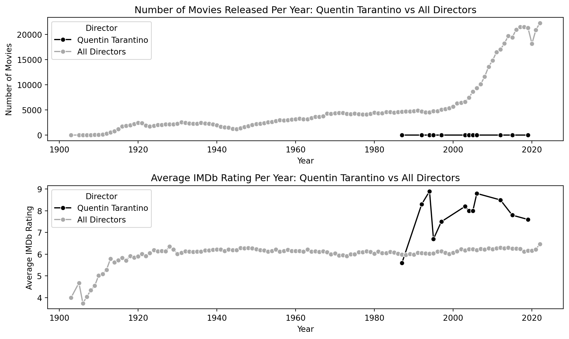

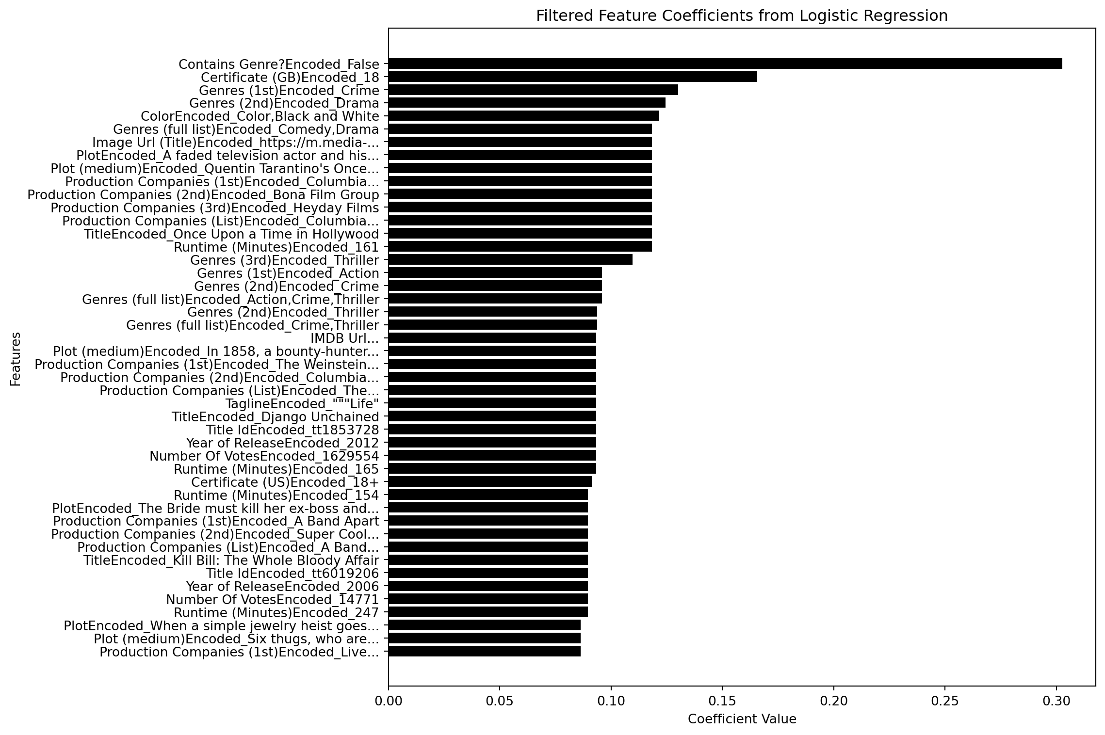
LASSO Modeling: Extract Features for Binary Outcome

# Use Spark SQL to filter Quentin Tarantino's movies and add high rating binary label
query = """
SELECT *, CASE WHEN CAST(`IMDB Rating` AS INT) >= 7.0 AND `Person Name` = 'Quentin Tarantino'    THEN 1 ELSE 0 END AS label
FROM movies
WHERE  `What did they do ?` = 'director'

"""
filtered_df = spark.sql(query)
# filtered_df = filtered_df.dropna()
# filtered_df = filtered_df.distinct()

# # Create a list of string-type columns from the updated filtered_df, excluding 'label'
# string_features = [field.name for field in filtered_df.schema.fields 
#                   if isinstance(field.dataType, StringType) and field.name != "label"]


filtered_df = filtered_df.drop("IMDB Rating")

from pyspark.sql.functions import col, approx_count_distinct
from pyspark.sql.types import StringType, IntegerType, DoubleType

# Fill missing values for string and numeric types separately
string_columns = [field.name for field in filtered_df.schema.fields if isinstance(field.dataType, StringType)]
numeric_columns = [field.name for field in filtered_df.schema.fields if isinstance(field.dataType, (IntegerType, DoubleType))]

# Fill missing values
filtered_df = filtered_df.na.fill("missing", subset=string_columns)
filtered_df = filtered_df.na.fill(0, subset=numeric_columns)

# Identify columns with more than one distinct non-null value
valid_columns = []
for column in filtered_df.columns:
    try:
        distinct_count = filtered_df.filter(col(column).isNotNull()).agg(approx_count_distinct(column)).collect()[0][0]
        if distinct_count > 1:
            valid_columns.append(column)
    except Exception as e:
        print(f"Skipping column {column} due to error: {e}")

# Keep only valid columns
filtered_df = filtered_df.select(*valid_columns)

# # Check schema after filtering
# filtered_df.printSchema()

# # Get total rows
# total_rows = filtered_df.count()

# # Define partition size and calculate the number of partitions
# target_rows_per_partition = 10000
# num_partitions = (total_rows // target_rows_per_partition) + (1 if total_rows % target_rows_per_partition != 0 else 0)

# # Repartition based on the calculated number of partitions
# filtered_df = filtered_df.repartition(num_partitions)

# Check the number of partitions
print(f"Number of partitions after repartitioning: {filtered_df.rdd.getNumPartitions()}")
filtered_df.show(5)

Number of partitions after repartitioning: 38
+------------+----------------+----------------+---------------+---------------+----------------------------+---------+-------------+------------+------------+------------+--------------------+--------------------+--------------------+--------------------+------------------+--------------------+--------------+--------------------+--------------------+--------------------------+--------------------------+--------------------------+---------------------------+-------------+--------------------+--------------------+---------+---------------+---------------+-----------------+-----+
|Best Picture|Certificate (GB)|Certificate (US)|          Color|Contains Genre?|Contains Production Company?|Continent|      Country|Genres (1st)|Genres (2nd)|Genres (3rd)|  Genres (full list)|   Image Url (Title)|   IMDB Url (Person)|    IMDB Url (title)|          Language|         Person Name|Person Name ID|                Plot|       Plot (medium)|Production Companies (1st)|Production Companies (2nd)|Production Companies (3rd)|Production Companies (List)|       Region|             Tagline|               Title| Title Id|Year of Release|Number Of Votes|Runtime (Minutes)|label|
+------------+----------------+----------------+---------------+---------------+----------------------------+---------+-------------+------------+------------+------------+--------------------+--------------------+--------------------+--------------------+------------------+--------------------+--------------+--------------------+--------------------+--------------------------+--------------------------+--------------------------+---------------------------+-------------+--------------------+--------------------+---------+---------------+---------------+-----------------+-----+
|     missing|         missing|         missing|          Color|          False|                       False| Americas|    Argentina| Documentary|     missing|     missing|         Documentary|https://m.media-a...|https://www.imdb....|https://www.imdb....|Spanish; Castilian|      Willi Behnisch|     nm0066960|             missing|             missing|        Viada Producciones|                   missing|                   missing|       Viada Produccione...|South America|             missing|Cantata de las co...|tt0363499|           2003|              8|               52|    0|
|     missing|         missing|         missing|          Color|          False|                       False| Americas|United States|      Sci-Fi|      Horror|    Thriller|Sci-Fi,Horror,Thr...|https://m.media-a...|https://www.imdb....|https://www.imdb....|           English|    'Evil' Ted Smith|     nm0810107|Two demon hunters...|             missing|           Pirate Pictures|                   missing|                   missing|        Pirate Pictures; ; |North America|There's bad blood...|Guardian of the R...|tt0361679|           2004|            311|              111|    0|
|     missing|               U|        Approved|Black and White|           True|                       False| Americas|United States|      Comedy|       Music|     missing|        Comedy,Music|https://m.media-a...|https://www.imdb....|https://www.imdb....|           English|A. Edward Sutherland|     nm0840042|A Paramount Studi...|Pop, a security g...|        Paramount Pictures|                   missing|                   missing|       Paramount Picture...|North America|The Musical Comed...|Star Spangled Rhythm|tt0035379|           1942|            649|               99|    0|
|     missing|         missing|         missing|Black and White|          False|                       False| Americas|United States|       Drama|     missing|     missing|               Drama|https://m.media-a...|https://www.imdb....|https://www.imdb....|           missing|A. Edward Sutherland|     nm0840042|Tom Blackford is ...|Tom Blackford is ...|      Famous Players-La...|                   missing|                   missing|       Famous Players-La...|North America|"""Here is a stor...|      Coming Through|tt0015699|           1925|        missing|               70|    0|
|     missing|         missing|         missing|Black and White|           True|                       False| Americas|United States|      Comedy|     missing|     missing|              Comedy|https://m.media-a...|https://www.imdb....|https://www.imdb....|           English|A. Edward Sutherland|     nm0840042|Prince Alexis is ...|Prince Alexis is ...|        Paramount Pictures|                   missing|                   missing|       Paramount Picture...|North America|Enough laughs to ...|    A Regular Fellow|tt0016280|           1925|        missing|               50|    0|
+------------+----------------+----------------+---------------+---------------+----------------------------+---------+-------------+------------+------------+------------+--------------------+--------------------+--------------------+--------------------+------------------+--------------------+--------------+--------------------+--------------------+--------------------------+--------------------------+--------------------------+---------------------------+-------------+--------------------+--------------------+---------+---------------+---------------+-----------------+-----+
only showing top 5 rows

from pyspark.sql import functions as F
from pyspark.sql.types import IntegerType, DoubleType
from pyspark.ml.feature import StringIndexer, OneHotEncoder, VectorAssembler, StandardScaler
from pyspark.ml import Pipeline
from pyspark.ml.classification import LogisticRegression
from pyspark.ml.tuning import CrossValidator, ParamGridBuilder
from pyspark.ml.evaluation import BinaryClassificationEvaluator, MulticlassClassificationEvaluator

try:
    # Step 1: Convert relevant columns to numeric types
    filtered_df = (filtered_df
                   .withColumn("Year of Release", F.col("Year of Release").cast(IntegerType()))
                   .withColumn("Number Of Votes", F.col("Number Of Votes").cast(DoubleType()))
                   .withColumn("Runtime (Minutes)", F.col("Runtime (Minutes)").cast(DoubleType())))
except Exception as e:
    print(f"Error during data type conversion: {e}")

try:
    # Step 2: Extract string and numerical features
    string_features = [field.name for field in filtered_df.schema.fields 
                       if isinstance(field.dataType, StringType)]
except Exception as e:
    print(f"Error extracting string features: {e}")

try:
    # Step 3: Indexing string features
    indexers = [
        StringIndexer(inputCol=col, outputCol=f"{col}Index", handleInvalid="skip") 
        for col in string_features
    ]
except Exception as e:
    print(f"Error creating indexers for string features: {e}")

try:
    # Step 4: Encoding indexed string features
    encoders = [
        OneHotEncoder(inputCol=f"{col}Index", outputCol=f"{col}Encoded") 
        for col in string_features
    ]
except Exception as e:
    print(f"Error creating encoders for string features: {e}")

try:
    # Step 5: Extract numerical features, excluding the label column
    numerical_features = [field.name for field in filtered_df.schema.fields 
                          if isinstance(field.dataType, (IntegerType, DoubleType)) and field.name != "label"]
except Exception as e:
    print(f"Error extracting numerical features: {e}")

try:
    # Step 6: Assemble both encoded string features and numerical features
    assembler = VectorAssembler(
        inputCols=[f"{col}Encoded" for col in string_features] + numerical_features,
        outputCol="features"
    )
except Exception as e:
    print(f"Error creating the VectorAssembler: {e}")

try:
    # Step 7: Add a scaler for numerical features to standardize them
    scaler = StandardScaler(inputCol="features", outputCol="scaledFeatures", withStd=True, withMean=False)
except Exception as e:
    print(f"Error creating the StandardScaler: {e}")

try:
    # Step 8: Create pipeline with indexing, encoding, feature assembly, and scaling
    pipeline = Pipeline(stages=indexers + encoders + [assembler, scaler])
except Exception as e:
    print(f"Error creating the Pipeline: {e}")

try:
    # Step 9: Transform the data
    prepared_data = pipeline.fit(filtered_df).transform(filtered_df)
except Exception as e:
    print(f"Error during pipeline transformation: {e}")

try:
    # Step 10: Define logistic regression model (Lasso)
    lasso_logistic = LogisticRegression(featuresCol="scaledFeatures", labelCol="label", 
                                        elasticNetParam=1.0, family="binomial",
                                        rawPredictionCol="rawPrediction",
                                        probabilityCol="probability",
                                        predictionCol="prediction")
except Exception as e:
    print(f"Error initializing the Logistic Regression model: {e}")

try:
    # Step 11: Set up the evaluator
    evaluator = BinaryClassificationEvaluator(labelCol="label", rawPredictionCol="rawPrediction")
except Exception as e:
    print(f"Error initializing the BinaryClassificationEvaluator: {e}")

try:
    # Step 12: Define parameter grid for cross-validation
    paramGrid = (ParamGridBuilder()
                 .addGrid(lasso_logistic.regParam, [0.1, 0.01])  # Example of Lasso tuning
                 .addGrid(lasso_logistic.elasticNetParam, [0.0, 1.0])  # Lasso vs Ridge
                 .build())
except Exception as e:
    print(f"Error creating the parameter grid for CrossValidator: {e}")

try:
    # Step 13: Set up cross-validation
    crossval = CrossValidator(estimator=lasso_logistic,
                              estimatorParamMaps=paramGrid,
                              evaluator=evaluator,
                              numFolds=10)  # 10-fold cross-validation
except Exception as e:
    print(f"Error setting up the CrossValidator: {e}")

try:
    # Step 14: Fit the model with cross-validation
    cv_model = crossval.fit(prepared_data)
except Exception as e:
    print(f"Error fitting the model using cross-validation: {e}")

try:
    # Step 15: Apply the cross-validation model to make predictions
    predictions = cv_model.transform(prepared_data)
except Exception as e:
    print(f"Error making predictions with the cross-validation model: {e}")

try:
    # Step 16: Evaluate model performance using AUC, Accuracy, Precision, and Recall

    # AUC (Area Under ROC Curve)
    auc = evaluator.evaluate(predictions)
    print(f"AUC: {auc}")

    # Calculate Accuracy using the prediction column
    accuracy = predictions.filter(predictions.label == predictions.prediction).count() / float(predictions.count())
    print(f"Accuracy: {accuracy}")

    # Precision and Recall Evaluators
    precision_eval = MulticlassClassificationEvaluator(labelCol="label", predictionCol="prediction", metricName="precision")
    recall_eval = MulticlassClassificationEvaluator(labelCol="label", predictionCol="prediction", metricName="recall")

    # Precision
    precision = precision_eval.evaluate(predictions)
    print(f"Precision: {precision}")

    # Recall
    recall = recall_eval.evaluate(predictions)
    print(f"Recall: {recall}")
except Exception as e:
    print(f"Error evaluating model performance: {e}")

best_model = cv_model.bestModel
# Access the coefficients from the best model
coefficients = best_model.coefficients.toArray()

# Retrieve the final feature names after one-hot encoding from the VectorAssembler metadata
expanded_feature_names = []

# Access the metadata for the assembled features column
metadata = prepared_data.schema["features"].metadata

# Extract the names of all features used in the VectorAssembler
if "ml_attr" in metadata and "attrs" in metadata["ml_attr"]:
    attrs = metadata["ml_attr"]["attrs"]

    # Combine attributes from binary and numeric features
    for attr_type in ["numeric", "binary"]:
        if attr_type in attrs:
            for attr in attrs[attr_type]:
                expanded_feature_names.append(attr["name"])

# Debug: Print the number of final expanded feature names and coefficients
print(f"Number of expanded feature names: {len(expanded_feature_names)}")
print(f"Number of coefficients: {len(coefficients)}")

# Ensure there is no mismatch between the number of expanded feature names and coefficients
if len(expanded_feature_names) == len(coefficients):
    # Create a dictionary of feature names and their corresponding coefficients
    feature_importance = {expanded_feature_names[i]: coefficients[i] for i in range(len(coefficients))}

    # Keep only positive coefficients
    positive_feature_importance = {feature: coef for feature, coef in feature_importance.items() if coef > 0}

    # Sort the features by absolute value of the coefficients
    sorted_positive_feature_importance = sorted(positive_feature_importance.items(), key=lambda x: abs(x[1]), reverse=True)

    # Display the sorted feature importance for positive coefficients only
    print("Detailed Feature Importance (positive coefficients only, sorted by absolute value):")
    for feature, coef in sorted_positive_feature_importance:
        print(f"Feature: {feature}, Coefficient: {coef}")
else:
    print("There is still a mismatch between the number of expanded feature names and coefficients. Please check the data pipeline.")

import textwrap
import matplotlib.pyplot as plt
import seaborn as sns
max_len = 50  # Maximum feature name length before truncating

# Initialize a list to store the wrapped feature names
wrapped_features = []

# Loop through each feature and coefficient
for feature, coef in filtered_feature_coeff_df:
    if len(feature) > max_len:  # If feature name is longer than the max length
        # Wrap/shorten the feature name
        wrapped_feature = textwrap.shorten(feature, width=max_len, placeholder="...")
        wrapped_features.append((wrapped_feature,coef))
    else:
        wrapped_features.append((feature,coef))

# Sort features by coefficient values for better visualization
sorted_feature_coeff_df = sorted(wrapped_features, key=lambda x: x[1], reverse=True)[:50]
sorted_features, sorted_coefficients = zip(*sorted_feature_coeff_df)

# Set a color palette using seaborn
colors = ['k' if coeff > 0 else 'darkgrey' for coeff in sorted_coefficients]

# Plot the coefficients with color palette
plt.figure(figsize=(12, 8))
plt.barh(sorted_features, sorted_coefficients, color=colors)
plt.xlabel('Coefficient Value')
plt.ylabel('Features')
plt.title('Filtered Feature Coefficients from Logistic Regression')

# Invert the y-axis to make the biggest bar appear at the top
plt.gca().invert_yaxis()

plt.tight_layout()
plt.show();