Difference in Differences with LASSO

This analysis comes from the “Introductory Econometrics: A Modern Approach, 7e’’ by Jeffrey M. Wooldridge” book. I’ll be looking at the Difference-in-Difference estimator along with applying a variable selection model.

Description: Wooldridge Source: K.A. Kiel and K.T. McClain (1995), “House Prices During Siting Decision Stages: The Case of an Incinerator from Rumor Through Operation,” Journal of Environmental Economics and Management 28, 241-255. Professor McClain kindly provided the data. This is a subset of the full dataset.

The Policy Problem

RESEARCH QUESTION: Does a new garbage incinerator have an affect on home value ?

The construction of a garbage incinerator started in 1981, but it was not until 1985 that it became operational. There were rumors in 1978 that a new garbage incinerator would be built, and it was assumed that the construction and operation of the incinerator would have a negative impact on the value of homes located nearby. Therefore, it was hypothesized that the value of certain homes near the incinerator would be negatively affected. This dataset comprises a random sample of house prices that were sold in 1978 as compared to those sold in 1981.

HYPOTHESIS 1: Home values decrease near a garbage incinerator relative to those located further away.

\[ \beta_{i} < 0, \ \ i = 1 \]

Data

Variable name	Description
year:	1978 or 1981
age:	age of the house
agesq:	age^2
nbh:	neighborhood, 1-6
cbd:	dist. to cent. bus. dstrct, ft
intst:	dist. to interstate, ft.
lintst:	log(intst)
price:	selling price
rooms:	# rooms in house
area:	square footage of house
land:	square footage lot
baths:	# bathrooms
dist:	dist. from house to incin., ft.
ldist:	log(dist)
wind:	prc. time wind incin. to house
lprice:	log(price)
y81:	=1 if year == 1981
larea:	log(area)
lland:	log(land)
y81ldist:	y81*ldist
lintstsq:	lintst^2
nearinc:	=1 if dist <= 15840
y81nrinc:	y81*nearinc
rprice:	price, 1978 dollars
lrprice:	log(rprice)

# This removes everything from the R environment
rm(list = ls())
# Call the dataset from the Wooldridge package
data('kielmc')
# Name the data as df
df<-kielmc

mean_price<-mean(df$price)
median_price<-median(df$price)
ggplot(df) +
  aes(x = price) +
  geom_histogram(bins = 30L, fill = "#345178", col = "white") +
  geom_vline(xintercept = mean_price, linewidth = 2, linetype = 5)+
  geom_vline(xintercept = median_price, linewidth = 4, color = "red")+
  theme_minimal() +
  theme(panel.grid.minor = element_blank())+
  scale_x_continuous(labels = scales::dollar_format())+
  labs(x = "Price of House",
       title = "House Prices in the Area")+
  theme(panel.grid.minor = element_blank())+
  theme(plot.title = element_text(hjust = 0.5))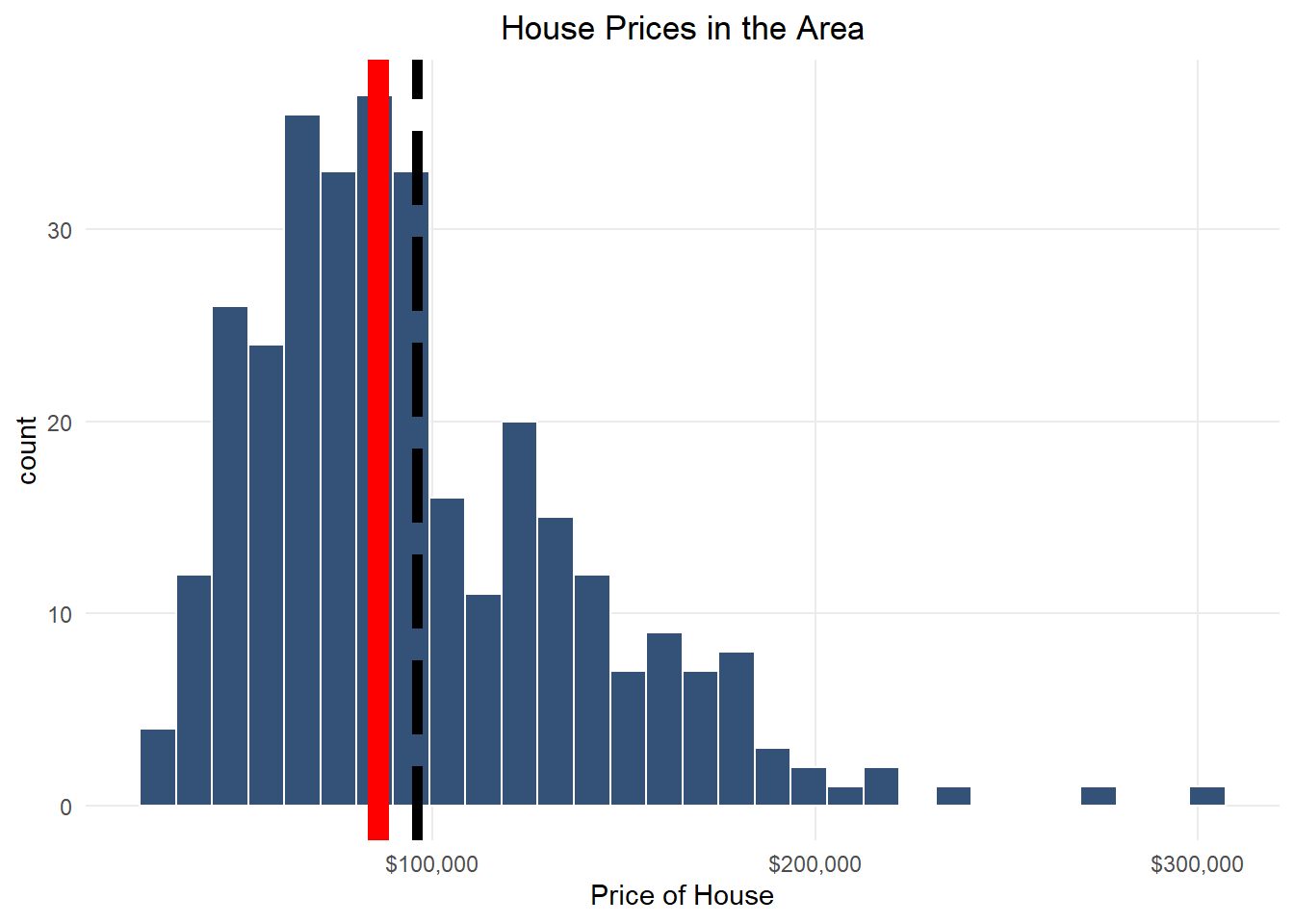

Figure 1

The data presented in Figure 1 provides valuable insights into the pricing patterns in the area. The chart indicates that the distribution of house prices is skewed towards the right, with a long tail. The vertical black and red lines on the chart suggest that the mean value of house prices is higher than the median value. These observations can help us understand how the prices of houses are determined in the area.

df %>%
  mutate(
    intervention = ifelse(nearinc == 1, "Near the Garbage Incinerator",
                          "Not Near the Garbage Incinerator")
  ) %>%
  ggplot(.,
         aes(x = price,
             y = intervention,
             fill = intervention)) +
  stat_density_ridges(quantile_lines = TRUE, quantiles = 2, scale = 3, color = "white")+
  scale_fill_manual(values = c("#00204D", "#D8D4B7"), guide = "none") + 
  scale_x_continuous(labels = scales::dollar_format())+
  labs(x = "Price of House",
       y = "Intervention")+
  theme_minimal() +
  theme(panel.grid.minor = element_blank())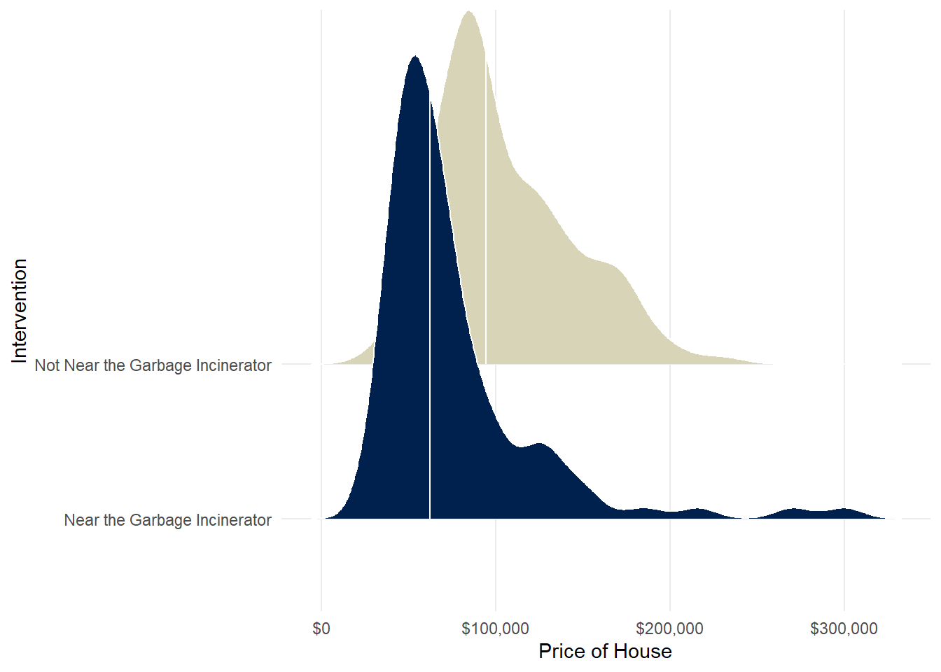

Figure 2

Figure 2 presents some interesting findings regarding the distribution of prices by intervention. The graph displays the median using the white vertical line. It is surprising to note that the most expensive house is located near the garbage incinerator, which indicates that the incinerator was placed in an area with lower home values.

out<-df %>%
  group_by(nearinc,year)%>%
  summarise(
    avg_price = mean(price,na.rm=T),
    median = median(price,na.rm=T)
  )


ggplot(out) +
  aes(
    x = year,
    y = avg_price,
    fill = nearinc,
    group = nearinc
  ) +
  geom_tile() +
  scale_fill_gradient() +
  scale_y_continuous(labels=scales::dollar_format())+
  theme_minimal()+
  labs(title = "Average House price relative to Incinerator between 1978 and 1981 ",
       x = "Year", y = "Average Home Price") +
  theme(plot.title = element_text(hjust = 0.5),
        axis.text=element_text(size=12),
        axis.title=element_text(size=12))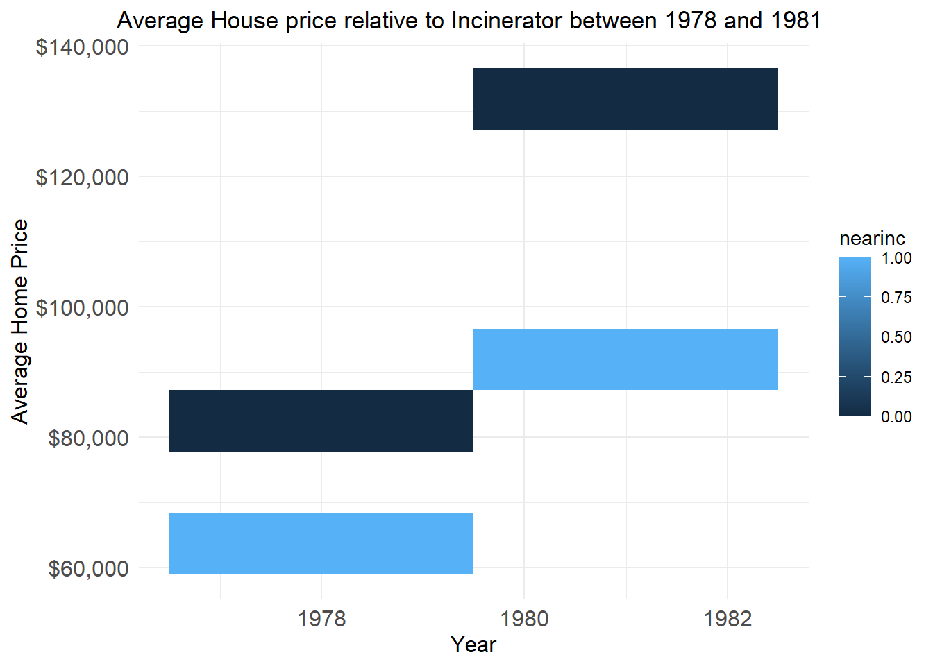

Figure 3

Figure 3 highlights a significant difference in the average home value for houses located near the incinerator. The data indicates that even before the construction of the incinerator, there was a visible difference in the value of houses situated near it. These findings can help us understand the impact of the incinerator on the value of properties in the area.

Initial Model

reg1<-lm( price ~ nearinc, data=df )
reg2<-lm( price ~ nearinc*y81, data=df )
reg3<-lm( price ~ nearinc*y81+age+agesq, data=df )
msummary(list("reg1" = reg1,"reg2" = reg2, "reg3" = reg3), vcov = "HC1",
         stars = c('*' = .1, '**' = .05, '***' = .01))

	reg1	reg2	reg3
* p < 0.1, ** p < 0.05, *** p < 0.01
(Intercept)	104905.164***	82517.228***	90270.430***
	(2601.093)	(1882.391)	(1904.186)
nearinc	-29440.060***	-18824.370***	14032.888*
	(5339.538)	(5996.470)	(7775.849)
y81		49385.155***	52258.755***
		(4275.932)	(3529.873)
nearinc × y81		-21131.762**	-32817.364***
		(10070.705)	(8717.956)
age			-1735.145***
			(201.369)
agesq			10.028***
			(1.448)
Num.Obs.	321	321	321
R2	0.098	0.356	0.547
R2 Adj.	0.095	0.350	0.540
AIC	7735.8	7631.4	7522.5
BIC	7747.1	7650.3	7548.9
Log.Lik.	-3864.905	-3810.707	-3754.256
F	30.400	52.113	98.279
RMSE	40997.37	34628.12	29043.86
Std.Errors	HC1	HC1	HC1

HC1 are Robust Standard Errors From STATA

The third model, with additional controls, gives a different estimate with decreased standard errors on the interaction between nearinc and y81. For the second model, we will use log prices to calculate the percentage change in house prices.

Second Model

reg1<-lm( log(price) ~ nearinc, data=df )
reg2<-lm( log(price) ~ nearinc*y81, data=df )
reg3<-lm( log(price) ~ nearinc*y81+age+agesq, data=df )
msummary(list("reg1" = reg1,"reg2" = reg2, "reg3" = reg3), vcov = "HC1",
         stars = c('*' = .1, '**' = .05, '***' = .01))

	reg1	reg2	reg3
* p < 0.1, ** p < 0.05, *** p < 0.01
(Intercept)	11.493***	11.285***	11.371***
	(0.025)	(0.025)	(0.023)
nearinc	-0.383***	-0.340***	0.007
	(0.053)	(0.062)	(0.070)
y81		0.457***	0.484***
		(0.040)	(0.032)
nearinc × y81		-0.063	-0.185**
		(0.095)	(0.077)
age			-0.018***
			(0.002)
agesq			0.000***
			(0.000)
Num.Obs.	321	321	321
R2	0.160	0.409	0.615
R2 Adj.	0.158	0.403	0.609
AIC	7634.8	7526.1	7392.3
BIC	7646.1	7545.0	7418.7
Log.Lik.	-162.034	-105.675	-36.785
F	51.901	67.170	129.554
RMSE	0.40	0.34	0.27
Std.Errors	HC1	HC1	HC1

HC1 are Robust Standard Errors From STATA

Here, we can see that the interaction between 1981 and being near the garbage incinerator in Model 3 decreased home value by almost 19%. We do have additional variables to include as controls. A selection model, like the LASSO, would be great to use. This model is a Penalized Regression model. The goal for the “least absolute shrinkage and selection operator,” or LASSO, is to minimize the sum of squared residuals and shrink the Beta coefficients. The LASSO also throws out certain coefficients, which makes it a variable selector.

What else could we include as controls for our model?

LASSO Regression Variable Selection

set.seed(1234)

df_split <- initial_split(df, strata = nearinc)
df_train <- training(df_split)
df_test <- testing(df_split)

It is necessary to separate the data into a training and testing dataset to predict. However, it’s essential to consider the skewed data on the price of housing. Also, we should be interested only in the variables that significantly affect the cost of housing. To ensure that the price balance between the training and testing data is maintained, we can use the data input in the initial_split function.

set.seed(1234)

office_rec <- recipe(lprice ~ ., data = df_train) %>%
  step_rm(lrprice, rprice, price)%>%
  step_zv(all_numeric(), -all_outcomes()) %>%
  step_normalize(all_numeric(), -all_outcomes())

office_prep <- office_rec %>%
  prep(strings_as_factors = FALSE)

set.seed(1234)
lasso_spec <- linear_reg(penalty = 0.1, mixture = 1) %>%
  set_engine("glmnet")

wf <- workflow() %>%
  add_recipe(office_rec)

lasso_fit <- wf %>%
  add_model(lasso_spec) %>%
  fit(data = df_train)

lasso_fit %>%
  pull_workflow_fit() %>%
  tidy()

# A tibble: 22 × 3
   term        estimate penalty
   <chr>          <dbl>   <dbl>
 1 (Intercept)     11.4     0.1
 2 year             0       0.1
 3 age              0       0.1
 4 agesq            0       0.1
 5 nbh              0       0.1
 6 cbd              0       0.1
 7 intst            0       0.1
 8 lintst           0       0.1
 9 rooms            0       0.1
10 area             0       0.1
# ℹ 12 more rows

set.seed(1234)
office_boot <- bootstraps(df_train, strata = nearinc)

tune_spec <- linear_reg(penalty = tune(), mixture = 1) %>%
  set_engine("glmnet")

lambda_grid <- grid_regular(penalty(), levels = 50)

set.seed(1234)
doParallel::registerDoParallel()

lasso_grid <- tune_grid(
  wf %>% add_model(tune_spec),
  resamples = office_boot,
  grid = lambda_grid
)

set.seed(1234)

lasso_grid %>%
  collect_metrics() %>%
  ggplot(aes(penalty, mean, color = .metric)) +
  geom_errorbar(aes(
    ymin = mean - std_err,
    ymax = mean + std_err
  ),
  alpha = 0.5
  ) +
  geom_line(size = 1.5) +
  facet_wrap(~.metric, scales = "free", nrow = 2) +
  scale_x_log10() +
  theme(legend.position = "none")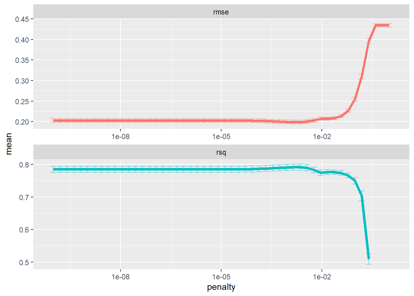

set.seed(1234)

lowest_rmse <- lasso_grid %>%
  select_best(metric = "rmse")

final_lasso <- finalize_workflow(
  wf %>% add_model(tune_spec),
  lowest_rmse
)


final_lasso %>%
  fit(df_train) %>%
  pull_workflow_fit() %>%
  vi(lambda = lowest_rmse$penalty) %>%
  mutate(
    Importance = abs(Importance),
    Variable = fct_reorder(Variable, Importance)
  ) %>%
  ggplot(aes(x = Importance, y = Variable, fill = Sign)) +
  geom_col() +
  scale_x_continuous(expand = c(0, 0)) +
  labs(y = NULL)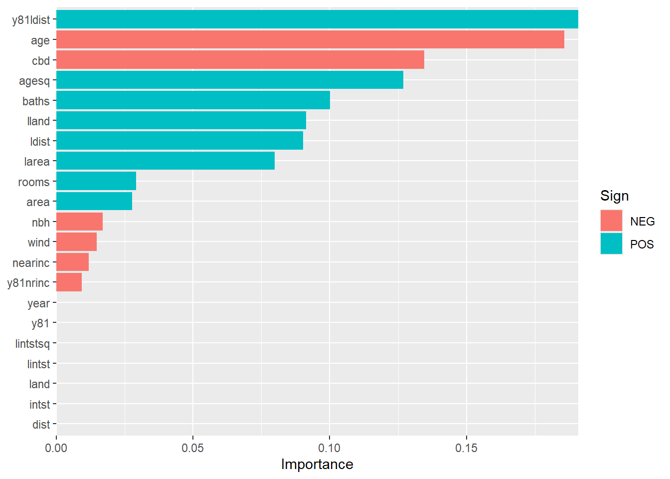

variable<-final_lasso %>%
  fit(df_train) %>%
  pull_workflow_fit() %>%
  vi(lambda = lowest_rmse$penalty) %>%
  mutate(
    Importance = abs(Importance),
    Variable = fct_reorder(Variable, Importance)
  ) %>%
  filter(Importance != 0) %>%
  pull(Variable)

new_df <- df %>%
  select(all_of(variable)) %>%
  mutate(lprice = df$lprice)

This part shows that the new_df will include all the variables kept from the LASSO regression model. Next, these variables will be included in OLS. This will be compared to the other simpler models. The standard errors will use the clustered method.

reg1<-lm( lprice ~ nearinc, data=new_df )
reg2<-lm( lprice ~ nearinc + y81nrinc, data=new_df )
lasso<-lm( lprice ~ ., data=new_df )
msummary(list("reg1" = reg1,"reg2" = reg2, "lasso" = lasso), vcovCL = "nearinc",
         stars = c('*' = .1, '**' = .05, '***' = .01))

	reg1	reg2	lasso
* p < 0.1, ** p < 0.05, *** p < 0.01
(Intercept)	11.493***	11.493***	7.136***
	(0.027)	(0.026)	(1.350)
nearinc	-0.383***	-0.547***	0.068
	(0.049)	(0.058)	(0.058)
y81nrinc		0.394***	-0.071
		(0.080)	(0.051)
y81ldist			0.040***
			(0.003)
age			-0.008***
			(0.001)
cbd			0.000***
			(0.000)
agesq			0.000***
			(0.000)
baths			0.094***
			(0.028)
lland			0.108***
			(0.025)
ldist			0.166**
			(0.074)
larea			0.109
			(0.166)
rooms			0.050***
			(0.017)
area			0.000
			(0.000)
nbh			-0.007
			(0.006)
wind			-0.003
			(0.007)
Num.Obs.	321	321	321
R2	0.160	0.220	0.800
R2 Adj.	0.158	0.215	0.791
AIC	330.1	308.7	-104.3
BIC	341.4	323.7	-44.0
Log.Lik.	-162.034	-150.327	68.165
F	60.977	44.725	87.401
RMSE	0.40	0.39	0.20

Clustered on Treatment Group

The power of machine learning is astonishing for predictive analytics. However, it can cause issues for causal inference when assessing the impact of the garbage incinerator. The LASSO model threw out one crucial variable, the y81 variable. But, the model kept the interaction of the y81 and nrinc variable.

The third model above includes all the variables selected by the LASSO regression model. This model increased the Adjusted R Squared. However, it needs to be adjusted regarding proper identification. For causal inference, identification should come before the actual analysis. This demonstrates the reason why.

Identification

The identification process guides the analysis in properly discovering the tested policy. This is taken from previous research and theory combined with the illustration of the data-generating process. A directed acyclic graph (DAG) sets up a solid workflow of our model to demonstrate the isolated path from policy to outcome.

Here, time is shown to asses the policy, with a compaison of before and after house prices. So, the y81 variable needs to be included in the model.

reg1<-lm( lprice ~ nearinc, data=new_df )
reg2<-lm( lprice ~ nearinc+y81+y81nrinc+land+area+dist, data=df )
reg3<-lm( lprice ~ nearinc+y81+y81nrinc+lland+larea+ldist, data=df )
msummary(list("reg1" = reg1,"reg2" = reg2, "reg3" = reg3), vcovCL = "nearinc",
         stars = c('*' = .1, '**' = .05, '***' = .01))

	reg1	reg2	reg3
* p < 0.1, ** p < 0.05, *** p < 0.01
(Intercept)	11.493***	10.517***	4.892***
	(0.027)	(0.088)	(0.624)
nearinc	-0.383***	-0.199***	-0.032
	(0.049)	(0.060)	(0.064)
y81		0.386***	0.421***
		(0.036)	(0.034)
y81nrinc		-0.032	-0.097
		(0.064)	(0.061)
land		0.000**
		(0.000)
area		0.000***
		(0.000)
dist		0.000
		(0.000)
lland			0.128***
			(0.024)
larea			0.597***
			(0.045)
ldist			0.048
			(0.055)
Num.Obs.	321	321	321
R2	0.160	0.663	0.694
R2 Adj.	0.158	0.656	0.688
AIC	330.1	47.5	16.1
BIC	341.4	77.7	46.3
Log.Lik.	-162.034	-15.744	-0.062
F	60.977	102.759	118.677
RMSE	0.40	0.25	0.24

Clustered on Treatment Group

new_df <- df %>%
  select(all_of(variable)) %>%
  mutate(lprice = df$lprice,
        y81 = df$y81)


lasso<-lm( lprice ~ ., data=new_df )
lasso2<-lm( lprice ~ .-cbd-agesq-area-wind-y81ldist, data=new_df )
reg4<-lm( lprice ~ nearinc+y81+y81nrinc+lland+larea+ldist, data=df )

msummary(list("lasso"=lasso,"lasso2"=lasso2,"reg4"=reg4), vcovCL = "nearinc",
         stars = c('*' = .1, '**' = .05, '***' = .01))

	lasso	lasso2	reg4
* p < 0.1, ** p < 0.05, *** p < 0.01
(Intercept)	6.420***	6.433***	4.892***
	(1.395)	(0.615)	(0.624)
y81ldist	-0.133
	(0.090)
age	-0.008***	-0.002***
	(0.001)	(0.000)
cbd	0.000***
	(0.000)
agesq	0.000***
	(0.000)
baths	0.093***	0.132***
	(0.027)	(0.026)
lland	0.110***	0.080***	0.128***
	(0.025)	(0.021)	(0.024)
ldist	0.223***	0.065	0.048
	(0.079)	(0.051)	(0.055)
larea	0.125	0.351***	0.597***
	(0.165)	(0.052)	(0.045)
rooms	0.051***	0.059***
	(0.017)	(0.017)
area	0.000
	(0.000)
nbh	-0.006	-0.017***
	(0.006)	(0.006)
wind	-0.006
	(0.007)
nearinc	0.131**	0.085	-0.032
	(0.067)	(0.058)	(0.064)
y81nrinc	-0.222**	-0.093*	-0.097
	(0.094)	(0.052)	(0.061)
y81	1.745*	0.413***	0.421***
	(0.912)	(0.029)	(0.034)
Num.Obs.	321	321	321
R2	0.802	0.783	0.694
R2 Adj.	0.793	0.776	0.688
AIC	-106.2	-86.3	16.1
BIC	-42.0	-41.0	46.3
Log.Lik.	70.080	55.153	-0.062
F	82.527	111.894	118.677
RMSE	0.19	0.20	0.24

Clustered on Treatment Group

anova(lasso,lasso2, reg4)

Analysis of Variance Table

Model 1: lprice ~ y81ldist + age + cbd + agesq + baths + lland + ldist + larea + rooms + area + nbh + wind + nearinc + y81nrinc + y81 Model 2: lprice ~ (y81ldist + age + cbd + agesq + baths + lland + ldist + larea + rooms + area + nbh + wind + nearinc + y81nrinc + y81) - cbd - agesq - area - wind - y81ldist Model 3: lprice ~ nearinc + y81 + y81nrinc + lland + larea + ldist Res.Df RSS Df Sum of Sq F Pr(>F)
1 305 12.145
2 310 13.329 -5 -1.1837 5.9451 2.902e-05 3 314 18.802 -4 -5.4730 34.3604 < 2.2e-16

---

Signif. codes: 0 ‘’ 0.001 ’’ 0.01 ’’ 0.05 ‘.’ 0.1 ’ ’ 1

The results indicate that the LASSO model with the y81 variable continues to outperform the other two models. The second model eliminates variables that are either already included in the model with the logarithm function or are not part of our DAG. The third model, however, stands out for its simplicity, which could potentially offer certain advantages. To compare all three, we can run an ANOVA. The results show the following:

LASSO vs. LASSO2 are significantly different. The variables excluded(CBD, ages, area, wind, and y81ldist) add significant predictive power. This is also true for the comparison of LASSO2 and reg4. Cross-validation will also be used to confirm these results.

# Model formulas
formula_model1 <- lprice ~ y81ldist + age + cbd + agesq + baths + lland + ldist + larea + rooms + area + nbh + wind + nearinc + y81nrinc + y81
formula_model2 <- lprice ~ nearinc + y81 + y81nrinc + lland + larea + ldist + age + baths + rooms + nbh
formula_model3 <- lprice ~ nearinc + y81 + y81nrinc + lland + larea + ldist

# Define cross-validation method (10-fold cross-validation)
train_control <- trainControl(method = "cv", number = 10)

# Train the models using cross-validation

# Model 1
cv_model1 <- train(formula_model1, data = df, method = "lm", trControl = train_control)

# Model 2
cv_model2 <- train(formula_model2, data = df, method = "lm", trControl = train_control)

# Model 3
cv_model3 <- train(formula_model3, data = df, method = "lm", trControl = train_control)


# Print results for each model
print(cv_model1)

Linear Regression 

321 samples
 15 predictor

No pre-processing
Resampling: Cross-Validated (10 fold) 
Summary of sample sizes: 289, 288, 290, 288, 289, 289, ... 
Resampling results:

  RMSE       Rsquared   MAE      
  0.2080967  0.7845689  0.1512256

Tuning parameter 'intercept' was held constant at a value of TRUE

print(cv_model2)

Linear Regression 

321 samples
 10 predictor

No pre-processing
Resampling: Cross-Validated (10 fold) 
Summary of sample sizes: 289, 288, 289, 289, 289, 290, ... 
Resampling results:

  RMSE       Rsquared   MAE      
  0.2124745  0.7690772  0.1547486

Tuning parameter 'intercept' was held constant at a value of TRUE

print(cv_model3)

Linear Regression 

321 samples
  6 predictor

No pre-processing
Resampling: Cross-Validated (10 fold) 
Summary of sample sizes: 289, 289, 288, 288, 290, 290, ... 
Resampling results:

  RMSE       Rsquared   MAE      
  0.2467578  0.6968864  0.1836055

Tuning parameter 'intercept' was held constant at a value of TRUE

Results

From above, the LASSO model performs the best based on the R2 and RMSE. This has the slightly highest r2 and lowest rmse. The second LASSO2 model is close. For this example, I’m going with the LASSO model.

The LASSO regression model, which is just OLS with the variables selected from the LASSO model, shows that homes near the garbage incinerator decreased in value by ~ 22% .  In 1978, when the rumor began about installing a garbage incinerator, house prices increased roughly ~ 13%. In 1981, this dropped to 1% during the incinerator’s construction. Using an Inverse Probability Weight (IPW) and rerunning a difference-in-differences model to compare the results to this analysis would be interesting. The IPW includes matching, which helps when we have differences in covariates between the treated and untreated groups. This method brings more balance to the covariates.

---